The Headless Studio
Chapter 1 — The Case for a Headless Studio
A headless studio turns musical decisions into data and audio-processing steps. Start with a complete example, then inspect the files each stage produces:
python -m pip install -r requirements.txt
python scripts/generate_portable_samples.py --piece afterimage --output-dir Tracks/demo
This example needs NumPy and SciPy. FFmpeg adds delivery exports. The following chapters explain optional instrument runtimes, sample maps, synthesis, arrangement, performance, mixing and publication. The complete scripts live in the repository; short fragments isolate the concept being discussed.
Take 47 is a diff
Here is a complete, honest description of how I changed the guitar sound on one of my songs:
-GUITAR_AMP = AMP_TWIN
+GUITAR_AMP = AMP_AC15
One line of code. I changed which amplifier the guitar plays through — from a Fender Twin to a Vox AC15 — the way you’d change any setting in any program: edit the variable, run it again. Ninety seconds later I had the same song, same performance, every note identical, through a different amp.
Not a performance like the last one. The same performance. When I couldn’t decide between the two amps, I generated both versions and listened blind. When I wondered whether the chorus effect belonged before the amp or after it, that was a one-line change too, and the answer took four minutes to settle beyond argument.
If you’ve ever used recording software — GarageBand, Ableton, Logic, any of the programs the industry calls DAWs (Digital Audio Workstations) — you know this is not how it normally goes. Changing your mind after the fact means clicking through the project, re-doing things by hand, and hoping you remember what else you touched. Your experiments live in the undo history and nowhere else.
My whole studio is a set of Python scripts. A song, for me, is a program
whose output is a finished audio file. This book is about how that studio
works and how to build your own — and you don’t need to be a Python expert
to follow along. If you can read a for loop and a function definition in
any language, you’re equipped; everything Python-specific gets explained
the first time it appears.
One note on the examples in this chapter. The amps, the bass and the drum machine comparison come from earlier guitar-driven work in the same studio, because they make the argument fastest. The two albums this book goes on to build — Sign-Off and The Quiet Hours — use synthesis and sampled instruments instead, and you’ll meet their actual sources from Chapter 5 onward. Same scripts, different band.
But first I owe you an argument for why anyone would do this.
What a DAW actually is
Strip the interface off any music production program and you find the same four machines inside:
- A scheduler — a list of what should happen when: play this note at this moment, trigger this drum sample at that moment.
- A plugin host — the part that loads instruments and effects (plugins) and pushes audio through them.
- A mixer — the part that combines many instrument tracks into one, each at its own volume.
- A renderer — the part that runs everything and writes the final audio file.
Everything else — the timeline you scroll, the piano roll, the faders — is user interface on top of those four functions. And the interface is the whole product: it’s what lets a musician who will never write a loop make records.
But here’s the thing about those four machines. A scheduler is a sorted list. A mixer is addition. A renderer is a loop. And the plugin host — the one genuinely hard piece of engineering — turns out to be something you can install with one command:
from pedalboard import load_plugin

amp = load_plugin("NeuralAmpModeler.vst3")   # a real guitar amp plugin
produced = amp(guitar_recording, 44100)      # audio in, amped audio out
That’s a real, professional-grade amplifier simulator — the same plugin
working guitarists use in Logic — loaded and running in two lines of
Python, no window anywhere. (The 44100 is the sample rate, which we’ll
properly meet in the next chapter; for now, it just means “CD-quality
audio.”)
Once I understood that plugins — the crown jewels of forty years of audio software — could be driven from a script, the rest of the DAW stopped looking necessary. What remained was a question: if the studio were a program, what would that buy you?
Buy-in #1: the performance that never has a bad night
Run one of my song scripts twice, and the two output files are identical. Not “sounds the same” — byte-for-byte identical. Programmers call this determinism: same input, same output, every time.
That sounds like a party trick until you see what it enables. Every choice in the song — every note, every volume level, every effect setting — is a line of code. So every experiment becomes a controlled experiment. When I compare the AC15 version against the Twin version, I know with complete certainty that the amp is the only difference. The drummer didn’t rush one take; there are no takes.
Even the “human” imperfections are deterministic. My bass and guitar parts get small random timing and volume variations — real hands drift, and music with zero drift sounds robotic. But the randomness comes from a random number generator with a fixed seed (a starting value that makes the “random” sequence repeatable). Take 47’s tiny stumble is identical to take 1’s, unless I choose to change one number and roll a new performance.
Determinism also makes curiosity cheap. Does the synth pad even earn its place in this song? Multiply the pad’s volume by zero, render, listen. Ninety seconds. When experiments cost that little, you stop settling questions by fatigue and start settling them by listening.
Buy-in #2: the studio that remembers why
Because a song is a text file, a song’s history is a version-control history. Mine reads like a producer’s notebook, except every entry is executable:
bass: added a distorted layer under the clean one, quiet — the clean
      bass alone got lost under the drums
drums: swapped LinnDrum for MFB-512 after comparing all eight machines
chorus: lead guitar enters 8 bars later; doubled the quiet section
Every one of those is a decision I can revisit, reverse, or branch from. What did the song sound like before I doubled the quiet section? Check out the old version and render it. What if the whole album used the smaller-sounding room? That’s a branch, and the experiment runs across twelve songs while I make dinner.
Ask what the equivalent is in a DAW: project files named
song_final_v3_REAL_final, and the reason the bass changed in March
existing only in your head. I’m not claiming version control makes better
music. I’m claiming memory does — and code is the only studio medium
that remembers everything, including intent.
Buy-in #3: the for-loop is a producer’s superpower
The moment that converted me wasn’t about sound quality at all. I needed to pick a drum machine for a song. I had drum sounds from eight real machines — the famous LinnDrum, the Roland TR-808, six others. The DAW way to choose is to swap sounds in by hand, audition two or three, get tired, settle. The script way is a loop: render the song’s actual beat, through the song’s actual effects, once per machine. Eight audio files, one blind listen, one clear winner.
And the winner was not the machine the genre’s history said it should be. It was better. I’d never have found it by hand, because by option four I’d have stopped looking.
That’s the general shape of the leverage: anything your script expresses as a setting — the amp, the drum kit, the tempo, the arrangement — becomes something you can try every version of, for the cost of a loop. A DAW asks: is this good? A script can ask: is this the best of everything I have?
And it compounds. The band I built for one song — the guitar rig, the human-timing engine, the shared room reverb — played the next song the day I wrote its chords. Both of the albums on my drive exist because the cost of one more song had fallen to: describe it, listen, revise.
What this costs you
Now the honest part, because the DAW’s interface is not a weakness — it’s the entire point of a DAW, and giving it up costs real things.
You lose immediacy. There’s no grabbing a knob while the music plays. My creative loop is edit → render → listen, and even at ninety seconds, that’s a different rhythm than turning a physical dial. Some ideas die in those ninety seconds. (Some survive because of them — being forced to listen to the whole section, rather than looping two bars forever, catches problems the DAW workflow hides. But the trade isn’t free.)
You lose recording. This book will not help you record a singer or mic a guitar cabinet. A code studio is an arrangement and production instrument: it plays sampled, synthesized, and simulated instruments with programmed performances. If your music is built on live takes, this pipeline can still be your sketchpad and your mixing back end — there’s a whole chapter on handing work between the script world and the DAW world — but the recording booth stays human.
You take on plumbing. Plugins built for the wrong kind of processor. Sample libraries in formats nobody documented. Libraries that won’t load for reasons that take an afternoon to diagnose. Several chapters of this book exist precisely because I lost those afternoons — you’re buying the afternoons back, but you should enjoy that kind of problem-solving to live here.
Who finds the trade worth it? Developers who make music and always felt the DAW wasn’t quite their instrument. Producers drowning in repetitive rendering work a loop should be doing. Tinkerers who want to know what the magic boxes actually do. And anyone building software that needs to produce music without a human at the controls.
The shape of the machine
Here is the entire studio this book builds, as one picture:
  the song, as data          sections, chords, patterns — plain lists
        │
  note events                one list of notes per band member
        │
  instruments                samplers, synths, sampled drums — one track each
        │
  effects                    each member's amp/pedal chain (real plugins)
        │
  the mix                    volumes, plus one shared "room" reverb
        │
  the record                 final file + per-instrument files for remixing
Every arrow is a plain function; every box is a chapter. Part I builds the instruments. Part II assembles the band. Part III makes an album with it and ships it.
One warning before we start: the first time you run a script and a finished song comes out — mixed, warm, breathing — the DAW in your dock starts to look strange, like a fax machine after email. I take no responsibility for what happens to your old projects after that.
Let’s build the instruments.
Next — Chapter 2: Rendering Note Events with FluidSynth.
Chapter 2 — Rendering Note Events with FluidSynth
Somewhere between “here are the notes” and “here is an audio file” there has to
be an instrument. This chapter builds the smallest useful one, and along the way
finally explains the 44100 I waved at in Chapter 1.
The performance we hand the instrument doesn’t need to be a MIDI file. A list of tuples will do — a sample position, an action, a channel, a pitch, a velocity. Keeping it that plain is deliberate: the same list can drive a SoundFont synth or the studio’s own JSON-zone sampler, and later on it can drive both at once.
FluidSynth is one route to sound, and it’s optional. It wants three things,
which arrive from three different places: the native FluidSynth library, the
pyfluidsynth Python binding, and a SoundFont — a file full of recorded
instruments — whose terms permit what you intend to do with it. Installing the
binding gets you none of the other two, a fact I would like you to learn faster
than I did. The FluidSynth site has the
platform-specific installation guidance.
None of this is required to use the studio. The portable examples need only NumPy and SciPy, and The Quiet Hours plays prepared Salamander and VSCO samples. Pick the renderer that suits the source you want to hear; skipping this chapter’s setup costs you nothing later.
Audio is a list of numbers, very fast
Here is the whole of digital audio. A microphone’s diaphragm moves; we measure its position 44,100 times a second; we write those measurements down. Play them back at the same rate and the speaker traces the same movement. That’s it.
The 44,100 is the sample rate, in hertz — measurements per second — and 44.1 kHz is the CD standard, which is why it’s everywhere. Each measurement is a sample. A frame holds one sample for each channel, so a stereo frame is two numbers. Count in frames and the arithmetic stays honest: at 44,100 Hz, half a second is frame 22,050, no matter how many channels you have.
Everything in this book is an array of floating-point numbers with that shape. Effects are functions over those arrays. Mixing is addition. Once you’ve internalized that, most of the mystique drains out of audio software, which is either liberating or disappointing depending on your temperament.
Schedule in frames
Every event in the studio uses the same five fields:
(sample_position, 'on' or 'off', channel, midi_note, velocity)
The midi_note is a pitch number — 60 is middle C, and each step of 1 is one
semitone up or down the keyboard. velocity is how hard the note was struck,
from 1 to 127, a range MIDI inherited in 1983 and has never escaped.
Write your musical durations in seconds, convert both ends of each note to integer frames, then walk the list: pull audio up to the next event, apply the event, keep going. The event lands exactly on a frame boundary, and nothing has to wait around for a real-time audio device to catch up. This is the one genuine advantage of rendering offline — the clock is yours.
Here’s a complete single note, assuming an installed FluidSynth runtime and a SoundFont of your own:
import numpy as np
import fluidsynth
from scipy.io import wavfile

rate = 44100
end = 3 * rate
synth = fluidsynth.Synth(samplerate=float(rate))
try:
    sfid = synth.sfload('/path/to/instrument.sf2')
    if sfid < 0:
        raise RuntimeError('SoundFont failed to load')
    synth.program_select(0, sfid, 0, 0)
    events = [(0, 'on', 0, 60, 72), (rate, 'off', 0, 60, 0)]
    chunks = []
    position = 0
    for frame, action, channel, note, velocity in events:
        if frame > position:
            chunks.append(synth.get_samples(frame - position))
        if action == 'on':
            synth.noteon(channel, note, velocity)
        else:
            synth.noteoff(channel, note)
        position = frame
    chunks.append(synth.get_samples(end - position))
    audio = np.concatenate(chunks).reshape(-1, 2).astype(np.float32) / 32768.0
    assert np.isfinite(audio).all() and np.max(np.abs(audio)) > 0
    wavfile.write('soundfont-note.wav', rate, audio)
finally:
    synth.delete()
Read the loop and you’ll see the pattern that runs through the whole studio:
advance to the event, apply the event, repeat. The try/finally makes sure
the synth is released even if the SoundFont turns out to be missing, which it
will be at least once.
The note ends at one second but the file runs to three. Those two spare seconds are where the release lives — the sound a piano makes after you let go of the key. Cut the array at the note-off and you don’t get a clean ending, you get a click and a piano that’s been switched off at the wall.
The binding hands back 16-bit whole numbers, which is why we divide by 32768 to land in the −1.0 to 1.0 float range the rest of the studio uses. And if you go on to build something more general than a one-note demo, validate the rest of it: positions in sorted order, channel and pitch ranges in bounds, every note-on paired with a note-off, nothing scheduled past the end of the render. Every one of those has cost me an afternoon.
One instrument bus at a time
Several MIDI channels inside a single synth all emerge from the same output. If you want a separate bass fader and piano fader — and by Chapter 10 you will badly want them — render them to separate buses: separate arrays, from separate synth instances or from a renderer that hands you separate outputs on purpose. Mixing things together is easy and permanent. Keeping them apart costs almost nothing and buys you every later decision.
Overlapping notes at the same pitch are the classic trap. A MIDI note-off carries no voice identifier, so if two middle Cs are sounding, something has to decide which one it ends. The zone sampler accepts explicit voice IDs for exactly this; plain five-field events fall back on its documented first-in, first-out pairing. Don’t assume another synth resolves the ambiguity the same way, because the standard doesn’t make it.
Last, write things down. The SoundFont’s identity, the program you selected, the sample rate, the runtime version — recorded with the result. A reproducible event list is only half a performance; the instrument that received it is the other half, and it is the half that quietly changes when you upgrade something. And save the dry float WAV, so that when you change your mind about the mix next week, you’re reusing the actual performance instead of re-deriving it from instructions and hoping.
Next — Chapter 3: Processing Saved Audio with VST3 Effects.
Chapter 3 — Processing Saved Audio with VST3 Effects
A plugin is a function with an expensive haircut. Audio goes in, audio comes
out. Forty years of audio engineering sit inside the box, and the interface it
presents to us is process(samples) -> samples — which is why the box drops so
neatly into a Python studio despite having been built for a mouse.
That shape suggests the order of operations. Render the performance once, save it, then push it through as many effects as your patience allows without ever asking the instrument to play again. The instrument’s job is finished. The plugin’s job is a separate afternoon.
You don’t need plugins to start, and I’d rather you didn’t. The self-contained sketches run on NumPy and SciPy alone:
python -m pip install -r requirements.txt
python scripts/generate_portable_samples.py --piece open-window --output-dir Tracks/demo
That gives you dry buses, processed stems and a float mix — a small complete record, nothing downloaded. Reach for a plugin when there’s a particular sound you’re after: an amp model you already trust, a delay with a character you can’t be bothered to rebuild from first principles.
Put the plugin after the saved performance
The optional host installs with python -m pip install pedalboard. The plugin
itself is your problem. It has to match your operating system and your
processor architecture, and this repository ships nobody else’s software.
(Chapter 4 is entirely about what to do when that match can’t be made.)
Here is the whole idea, running a saved stereo float WAV through an effect. Substitute a path to something you actually have installed:
import numpy as np
from scipy.io import wavfile
from pedalboard import load_plugin

rate, frames = wavfile.read('Tracks/demo/open-window/dry/melody.wav')
assert frames.dtype == np.float32 and frames.ndim == 2
channels = frames.T.copy()                 # host layout: channels × frames
plugin = load_plugin('/path/to/effect.vst3')
processed = plugin(channels, rate)
assert np.isfinite(processed).all()
wavfile.write('Tracks/effected-melody.wav', rate, processed.T)
Two details in there will bite you if you skip past them.
Working in float means you never have to guess what scale the samples were stored at. A 16-bit integer WAV stores values from −32768 to 32767; a 24-bit one uses a different range again; float WAVs are simply −1.0 to 1.0 and always have been. Convert once, at the edges, and let everything in between be float.
And the transpose matters. SciPy hands you an array of frames, each holding its
channels — shape (frames, 2). The host wants channels, each holding its
frames — shape (2, frames). .T swaps those two axes, and .copy() makes the
result contiguous in memory, which some hosts insist on. Neither operation
touches the sample rate or changes a single number; they only change how the
numbers are arranged. Getting this backwards produces a result so mangled it’s
usually obvious, which is the one mercy of the situation.
Print plugin.parameters to see what the plugin exposes. Set the values you
care about deliberately, and write them down with the mix. Parameter names and
ranges belong to that specific plugin, so a setting that sounds right on my
amp model means precisely nothing on yours.
Preserve state and tails
Effects remember. A delay is holding echoes from a second ago. A compressor is partway through its envelope. An amp model has its own internal weather.
This matters because audio is often processed in blocks rather than all at once, and if you reset the plugin between blocks you’ll get a different result from processing the whole thing in one go — a delay that restarts, a compressor that keeps flinching. So when you process in blocks, use the host’s state-preserving mode, and leave enough trailing silence at the end for the effect to decay into. Then confirm it behaved, with the exact host and plugin versions you installed, because this is precisely the sort of thing that changes quietly between releases.
Some plugins also keep settings that never appear as automatable parameters —
a loaded impulse response, a model file, a mode switch buried in the UI. The
reliable move is to configure the plugin through its own interface, save a
preset, and load that. The repository’s music_engine/plugins.py has a Neural
Amp Modeler helper that understands one specific preset layout: an adapter for
a format I went and learned, not a general-purpose preset editor. If the format
changes, the helper needs re-checking before you trust it with a record.
Appendix C takes that apart byte by byte, for when the save-a-preset workflow
isn’t enough.
Keep the experiment comparable
Change one setting. Keep the dry performance fixed. Match the listening levels before you decide anything — a louder render sounds more detailed, more present, generally better, even when the only thing that improved was the gain. Everyone falls for this. Knowing about it helps less than you’d hope, so normalize the comparison instead of trusting yourself.
Save the processed bus as a float stem. If several instruments share a nonlinear effect — distortion, saturation, an amp — keep the combined output as a group stem as well. Separately processed inputs are not guaranteed to sum back to the same sound, and Chapter 12 shows exactly where and why that promise breaks.
One practical note: plugin loading in the shared engine is lazy, so the sampler and synthesis chapters never ask you to configure a host you didn’t want. And if a plugin insists on a runtime the rest of your studio can’t live with, you can push that one rendering step across a process boundary instead, which is the next chapter.
Next — Chapter 4: An Instrument Across a Process Boundary.
Chapter 4 — An Instrument Across a Process Boundary
Sooner or later you meet a plugin that is wonderful and impossible. It wants a different processor architecture, or a Python it refuses to share with yours, or native libraries that quietly break three other things you’d installed. The temptation is to bend the whole studio around it, and the studio will let you, right up until the day it doesn’t.
Don’t. Put the awkward instrument in its own process and talk to it through files. Write the events to JSON, ask a helper program to render them, read back the WAV it produces. Two processes that agree on a file format don’t have to agree on anything else — not their dependencies, not their Python version, not even their instruction set.
The shared implementation is scripts/music_engine/renderers.py. Your
arrangement code keeps calling one interface, while the helper quietly owns all
the awkwardness of one particular instrument.
Keep the boundary small
The parent sends a duration and a list of note records. The helper gets two paths: one JSON in, one WAV out. It sets up its own instrument, renders the whole performance and exits. The parent never learns which plugin parameter selects a preset, or where the helper found its native library, and that ignorance is the entire point — it’s what keeps the mess from spreading.
from music_engine import render_external_instrument

notes = [{'time': 0.0, 'duration': 0.8, 'pitch': 48, 'velocity': 72}]
audio = render_external_instrument(
    notes,
    total_seconds=3.0,
    python_path='/path/to/instrument-python',
    helper_path='/path/to/your-render-helper.py',
    sample_rate=44100,
)
if audio is None:
    raise RuntimeError('The selected instrument did not render')
Notice that these notes carry time and duration in seconds, not the
frame-position on/off pairs of Chapter 2. That’s deliberate: the bridge hands
whole notes across, and the helper decides how to schedule them. It suits a
process boundary better — fewer, larger messages, each one self-contained.
Those field names are a contract you’re proposing, not one the bridge enforces.
It passes the records through as JSON; your helper has to agree about the names
and their units. There is no universal instrument hiding in here, and if you
invent a pan field the bridge will carry it faithfully without ever knowing
what it means.
What comes back is channels by frames, the studio’s working layout. The bridge reads the helper’s WAV at whatever rate it was actually written, resamples if it must, promotes mono to stereo, and pads or trims to the duration you asked for. Which means: ask for a duration generous enough to hold your note releases and effect tails. Trimming happens at the end and has no sympathy for your reverb.
Match the runtime to the instrument
On a system with architecture translation — an Apple Silicon Mac running Intel binaries, say — the helper can run under a different architecture from its parent, provided you have a compatible interpreter, compatible native dependencies and a compatible plugin, all three. A process boundary is not a binary translator, and it certainly won’t carry a Windows-only plugin onto a Mac. All it does is stop two incompatible things from having to share one address space, which is quite enough.
The bridge takes an optional architecture argument for the macOS arch
command. Leave it unset for an ordinary subprocess. And get the helper working
on its own, from a terminal, before you wire it into a twelve-track album
render — unless you enjoy debugging by album, which takes about forty minutes
per attempt and teaches you very little.
For an instrument that streams from disk, give its library time to initialize and keep its state alive across render blocks. Tearing the processor down every block can cut sustained notes short, or send it back to reloading samples over and over while your render crawls. Those decisions belong inside the helper, where you can test them without running everything else.
Failure is a result you must handle
The bridge returns None when the interpreter isn’t available, when the note
list is empty, and when the helper reports failure. That’s a real outcome and
the caller has to do something about it: stop the render, or fall back to a
substitute you have written down somewhere.
What you must not do is quietly swap in a different instrument during a delivery build. It’s the most tempting line of code in this chapter and the worst — three months later, nobody can tell you what’s actually on the record. The chosen source belongs in the manifest, named, every time.
There is no timeout in the bridge. If you’re rendering unattended, wrap helpers that can hang in something with a bound on it, and keep their logs. Then check the WAV that came back: format, duration, finite samples, audible content. A zero exit code and thirty seconds of silence go together far more often than you would like.
None of this is needed for the portable sketches or either album render path. The process boundary exists for a sound that’s worth the trouble, and saved dry buses keep that setup well away from your routine mix comparisons.
Next — Chapter 5: Build a Sample Instrument from Your Own Sounds.
Chapter 5 — Build a Sample Instrument from Your Own Sounds
A sampler plays recordings at different pitches. That’s the whole trick, and it has been the whole trick since the 1970s. The recording might be a piano note, a struck wine glass, a drum hit, or a tone a program invented forty milliseconds ago — the player doesn’t care. Once the sound exists as a WAV file, the player only needs a map: which file answers this note, how fast should it play, and when should it stop?
Commercial sample libraries are enormous and genuinely clever, and they make this look like deep magic. It isn’t. It’s a folder of WAVs and a lookup table, and by the end of this chapter you’ll have built one and the mystery will be gone for good.
We’ll use sounds we generate ourselves. No commercial library, no undocumented file format, nothing to download and nothing to read a licence for first.
Make a small instrument
From the repository root, install the core dependencies and run:
python -m pip install -r requirements.txt
python scripts/generate_sampler_demo.py --output-dir Tracks/sampler-demo
What lands is an instrument and a short performance of it:
Tracks/sampler-demo/
  demo.wav
  instrument/
    manifest.json
    provenance.json
    tone-48-soft.wav
    tone-48-bright.wav
    tone-60-soft.wav
    tone-60-bright.wav
    tone-72-soft.wav
    tone-72-bright.wav
The script synthesizes all six recordings. Nothing is copied from a factory
library and no plugin is involved. The complete runnable implementation is
scripts/generate_sampler_demo.py; what follows explains the decisions inside
it rather than reprinting it line by line.
A recording is an array
Chapter 2 established the shape of digital audio: a sample rate of 44,100 means one second holds 44,100 amplitude values per channel. To lay out two seconds of time coordinates:
sample_rate = 44100
t = np.arange(sample_rate * 2, dtype=np.float64) / sample_rate
Every position in t is a moment, measured in seconds. A sine wave at some
frequency is then np.sin(2 * np.pi * frequency * t) — frequency being cycles
per second, so doubling it raises the pitch by exactly one octave. That
relationship is the reason the equal-tempered keyboard is built from twelfth
roots of two, and the reason this one line of arithmetic keeps reappearing:
frequency = 440 * 2 ** ((root - 69) / 12)
MIDI note 69 is the A at 440 Hz. Twelve semitone steps double the frequency. We generate roots at 48, 60 and 72 — an octave apart — so the player always has a nearby recording to work from, rather than stretching one sound across the entire keyboard and making everything above middle C sound like a chipmunk.
Give the sound a beginning and an ending
A tone that jumps straight from silence to a nonzero value clicks. You’ve heard it; it’s the sound of a waveform being cut with scissors. The fix is an envelope: an array of gains that shapes the amplitude over time. Ours uses a fast attack and a longer exponential decay:
envelope = (1 - np.exp(-t / .008)) * np.exp(-t / .65)
The first factor rises from zero — that’s the attack, eight milliseconds of it. The second falls toward zero, a decay with a time constant of 0.65 seconds. Multiply them and you get something struck and fading, which is a surprisingly large fraction of all the instruments there are. The full generator also fades the last 441 frames (ten milliseconds) to zero, so the file itself ends smoothly no matter where the decay got to.
Each pitch gets two timbres:
signal = .5 * envelope * (
    np.sin(2 * np.pi * frequency * t)
    + overtone * np.sin(4 * np.pi * frequency * t)
)
That second sine is an octave above the fundamental. Set overtone to .08
for the soft layer and .3 for the bright one. This is the point of a velocity
layer, and it’s worth being precise about: a harder-played note doesn’t just
get louder, it gets brighter, because hitting something harder excites more
high harmonics. A real multi-sampled instrument changes far more dramatically
between its soft and hard layers than our two sine waves do — but the principle
is identical, and now you can hear it working.
SciPy writes the source as floating-point WAV:
wavfile.write(path, sample_rate, signal.astype(np.float32))
That preserves working precision. It is not the format our albums are delivered in; conversion and mastering are their own stage, several chapters away.
Map each recording to a zone
A zone says where a recording gets used. Its key range selects pitches; its velocity range selects how hard the note was played. Both ranges are inclusive in this sampler.
{
  "name": "Tone 60 soft",
  "root": 60,
  "keylo": 54,
  "keyhi": 65,
  "vello": 1,
  "velhi": 79,
  "group": "Synth tones",
  "file": "tone-60-soft.wav"
}
Put every zone in a list and save it as manifest.json. The bright version
takes the same key range with velocities 80–127. The lower root covers notes
0–53 and the upper covers 66–127 — deliberately broad outer ranges that keep
the demonstration simple, though stretching one recording two octaves or more
sounds about as natural as you’d expect.
root is the pitch actually recorded in the file. To play MIDI 64 from a
root-60 recording, we read through the file faster:
ratio = 2 ** ((64 - 60) / 12)
About 1.26. The source position advances roughly 1.26 frames for every frame of output, which means fractional positions, which means interpolation. It also means the recording gets shorter as it gets higher: pitch and duration are welded together in a simple sampler, exactly as they were on tape. This is not a time-stretching instrument, and that limitation is why you record several roots instead of one.
Render a note
The shared engine exposes ZoneSampler, which reads the JSON manifest and
loads the WAVs it names. (You’ll also meet ExsSampler in the album renderer —
it’s the same class under a historical alias, kept so older scripts keep
working.)
from music_engine import ZoneSampler

sampler = ZoneSampler(
    "Tracks/sampler-demo/instrument",
    deterministic=True,
    stereo_output=True,
)
events = [
    (0, "on", 0, 64, 70),
    (round(0.6 * 44100), "off", 0, 64, 0),
]
audio = sampler.render(events, total_seconds=2.0)
Put this in a file inside scripts/, or set PYTHONPATH=scripts before
running it from elsewhere. The tuple fields are the five from Chapter 2:
integer sample position, event kind, channel, MIDI note, velocity. The note
starts immediately and releases at 0.6 seconds. The result has two channels and
88,200 frames — two seconds, as requested.
The implementation converts a source file’s sample rate before pitch shifting, centers unsigned 8-bit PCM correctly, and can preserve stereo sources. Small details, all three, and all three produce distinctive damage when got wrong: a transposition error, a DC offset, a collapsed stereo image. Our generated sources are mono, so stereo output simply duplicates them to both channels — it does not invent width that was never recorded.
A note-off starts the release envelope. A voice can also end because its recording ran out, which is what happens to short samples held for long notes. If another note starts while the first is still sounding, the arrays are added together rather than one stealing the other’s voice. Overlapping notes at the same pitch are paired first-in, first-out; an optional sixth tuple field supplies an explicit voice ID when a score needs to be certain which note-off belongs to which note.
Check the instrument by listening to its boundaries
The demo alternates soft and bright notes across the three roots, which is a start. But the interesting places are the seams. Play a slow phrase that crosses MIDI 53 to 54, and 65 to 66 — those are where the selected source changes. Then play the same note at velocity 79 and again at 80. You should hear the layer change as a change of character, not as an accidental jump in level. If it lurches, the instrument is miscalibrated, and no amount of mixing downstream will hide it.
When you build something larger, record more root notes before relying on
extreme transposition. Match recording levels deliberately. Trim starts
carefully — a few milliseconds of silence before the attack becomes audible
sloppiness in a fast passage. Leave enough decay for the longest note you
intend to play. And several alternate recordings of the same note will stop
repeated hits from sounding mechanically identical. The engine picks randomly
among equally matching zones unless you pass deterministic=True; it is not a
strict round-robin player, so it won’t guarantee each alternate gets its turn.
Keep the source record with the instrument
The generator writes provenance.json: a description of how the sounds were
synthesized, and a SHA-256 hash for each WAV. Those hashes establish which
files were used. They do not establish that you were allowed to use them, and
nothing in a JSON file ever will.
For your own recordings, keep your recording notes. For a third-party library, keep the actual licence and check that it permits your intended use — including redistribution, if you plan to share the instrument itself. Permission to use a sound in a finished composition is a different thing from permission to publish its individual samples or extract them into another player, and the second is much rarer than the first.
The project’s MIT licence covers its code and documentation. It does not relicense plugin libraries or anyone else’s recordings, and it can’t.
For this chapter you need none of that: the generator, the manifest and the sampler are a complete instrument you can open, read and change. Appendix B lists every manifest field.
Next — Chapter 6: Drum Machines Are Sample Players.
Chapter 6 — Drum Machines Are Sample Players
Here’s the thing nobody tells you: a drum machine is the instrument you built in Chapter 5, with the pitch-shifting turned off. One WAV per sound, triggered at scheduled positions. The LinnDrum that defined a decade of records is a sample player with a sequencer bolted to it.
Which means the interesting question isn’t how to play a kit. It’s how to choose one — and that turns out to be where most of the craft lives.
Audition in the mix, not in isolation
A kick drum auditioned on its own tells you almost nothing. What matters is what its tail does underneath a bass line, and you cannot hear that until the bass is playing. So when you’re choosing a kit, render the same section through every candidate and listen to it in context: same groove, same processing, same comparison level, so the kit is genuinely the only variable.
View the comparison of eight drum machine kicks
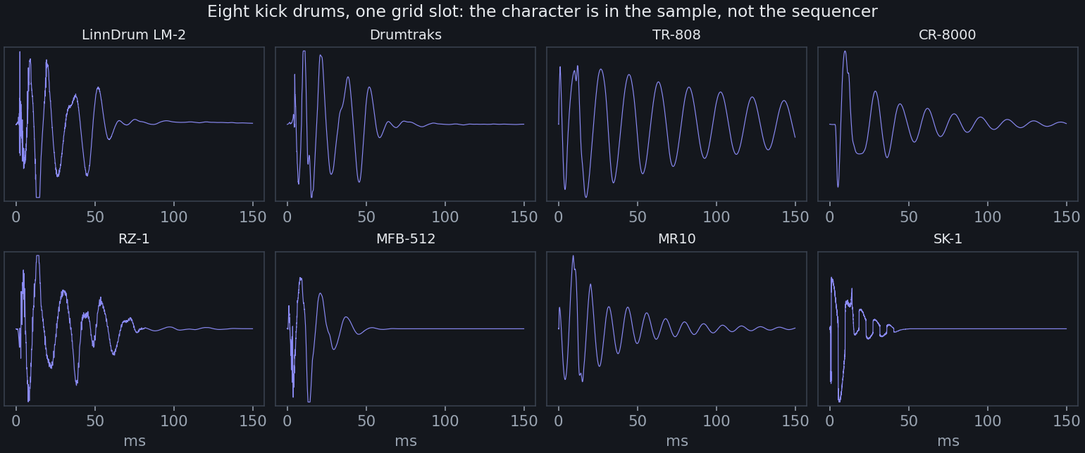
Look at how differently sampled kicks behave in attack, length and shape. That picture is not a ranking — it’s an argument for auditioning. A short kick may leave exactly the room a sustained bass needs. A longer one may be the low end the arrangement was missing. The waveform can’t tell you which, and neither can I.
This is also where Chapter 1’s for-loop argument stops being abstract. The DAW way to choose a kit is to swap sounds in by hand, get through three or four, get tired, and settle. The script way is a loop over candidate kit paths, and a blind listen at the end of it. The winner is frequently not the machine the genre’s history says it should be.
Treat each sample as a source with a format
Use recordings you made, or samples licensed for what you actually intend to do. Keep the source and its terms with the local kit — a download link is not a permission record, and you will not remember in a year. (The public repository doesn’t include the studio’s drum samples for exactly this reason.)
A WAV is not necessarily 16-bit, mono or 44.1 kHz, whatever the last ten files you opened happened to be. Drum samples in particular arrive from every era of computing, and some of them are older than you are. The shared reader handles integer and float PCM, centers unsigned 8-bit data, and resamples from whatever rate the file actually declares:
from music_engine.samplers import read_sample

rate = 44100
kick = read_sample('/path/to/your-kit/kick.wav', rate)
You get frames by channels for a stereo file, or a one-dimensional array for mono. Hold on to that distinction until you’ve decided deliberately how the kit should sit in the stereo image. Casting everything to float and dividing by 32768 works beautifully for exactly one encoding and silently mangles the rest — unsigned 8-bit audio treated that way comes out with a large DC offset and a click on every hit.
Fix the pattern before comparing kits
Write hit positions in beats, then convert to sample positions at the final tempo. Here’s a minimal mono example putting a kick down four times:
import numpy as np
from scipy.io import wavfile

bpm = 80
beat = 60 / bpm
mono = kick.mean(axis=1) if kick.ndim == 2 else kick
bus = np.zeros(round((4 * beat + 2) * rate), np.float32)
for beat_position, gain in [(0, .7), (1, .5), (2, .7), (3, .5)]:
    start = round(beat_position * beat * rate)
    count = min(len(mono), len(bus) - start)
    bus[start:start + count] += mono[:count] * gain
assert np.isfinite(bus).all()
wavfile.write('kit-pattern.wav', rate, bus)
The bus is four beats plus two spare seconds, because the last kick needs
somewhere to ring out. count clamps the copy so a long sample near the end of
the bus doesn’t run off the edge of the array. And += rather than = means
overlapping hits sum, the way two drums in a room would.
For a real audition harness, make the kit path the variable and reuse this same pattern for all of them. Keep an unprocessed version for diagnosis and a version through the actual drum bus for the musical decision; they answer different questions and you want both. Compare at matched listening levels, too — peak-normalizing two samples can still leave one obviously louder, and louder wins auditions it hasn’t earned.
Keep a stable rhythmic reference
Sign-Off renders its LM-2 kick, snare and closed hat at final-tempo positions. The pitched sources go off through the slowdown and warble path described in Chapter 7; the drum attacks skip that timing warp entirely. The kit can still be filtered and balanced however the track needs — it simply never leaves the beat.
That’s a musical decision with a routing consequence, and it’s worth stating as a principle: when something in your mix is going to drift, something else should stay put. The ear tolerates a great deal of instability as long as it has one thing to hold on to.
Contrast comes from the arrangement as much as the kit. Some tracks on the record run on a slow heartbeat pattern, some on a steady beat, some on nothing at all. One strong kit covers that whole range as long as the pattern and the texture around it have a reason for existing.
Check the dense passages and the transitions, not just the opening bar, which always sounds fine. Listen for kick and bass masking each other, for hats that turn tiring by the third minute, for tails clipped short by the export. Then, once you’ve chosen, save the performed drum bus with the other dry sources so your later mix comparisons reuse exactly the same hits.
Next — Chapter 7: Synthesis from a Few Sine Waves.
Chapter 7 — Synthesis from a Few Sine Waves
Every instrument so far has needed something from outside: a SoundFont, a plugin, a folder of recordings. This chapter needs nothing. A synthesized source starts from numbers, which means it starts from an equation you can read — and it means the first sound you make in this studio can be made on a laptop on a train with no internet.
The portable sketches are built this way. A few sine waves, some envelopes, a little noise, and out comes a complete arrangement:
python scripts/generate_portable_samples.py --piece open-window --output-dir Tracks/demo
Open Window is the sparse, beatless one. Afterimage and Night Transit add percussion and use different tempos, melodies and amounts of pitch movement. All three keep their composition and mix settings in a single file, so you can change something and hear the result before you’ve finished wondering about it.
Frequency, phase and time
We’ve met the arithmetic twice now, so here it is doing actual work:
import numpy as np
rate = 44100
note = 69
seconds = 2.0
frequency = 440 * 2 ** ((note - 69) / 12)
t = np.arange(round(seconds * rate)) / rate
signal = np.sin(2 * np.pi * frequency * t)
t is an array of times, one entry per frame. Multiplying time by frequency
counts cycles; multiplying by 2 * pi converts cycles into radians, which is
what np.sin expects. NumPy then evaluates the whole expression across the
entire array at once — no loop, no per-sample Python, which is the only reason
any of this runs fast enough to be enjoyable.
A single sine wave is one frequency and nothing else, which is why it sounds like a hearing test. Add another at twice the frequency and the sound gets brighter without its pitch changing:
signal += 0.28 * np.sin(2 * np.pi * 2 * frequency * t) * np.exp(-t * 3)
Note that the second harmonic decays faster than the fundamental. That’s the detail that makes it sound struck rather than synthetic: real instruments are brightest at the attack and mellow as they ring. A static blend of oscillators never does that, and the ear notices immediately even if it can’t say why.
An envelope makes a note
An oscillator has no idea when a note begins or ends; left alone it drones forever. An envelope is an array of gains that gives the sound a shape:
attack = 1 - np.exp(-t / 0.008)
decay = np.exp(-t / 0.6)
release = np.clip((seconds - t) / 0.05, 0, 1)
signal *= attack * decay * release
The attack rises quickly, the decay falls gradually, and the release pulls the final samples to zero — because cutting a waveform off partway through a cycle produces a click, and the click is louder than you expect. For a pad, slow the attack and the release down; the portable renderer keeps a different envelope for its sustained harmony voice.
These time constants are artistic parameters, not settings with correct values. Judge them over a real phrase rather than a single note, because a tone that sounds lovely on its own can have a tail that smears the note after it.
Place the sound on a bus
The studio’s working buses are channels by frames, so a stereo bus has shape
(2, frame_count). To place a mono note, we distribute it between left and
right. The portable renderer uses an equal-power pan:
pan = -0.2                         # -1 left, 0 center, +1 right
angle = (pan + 1) * np.pi / 4
stereo_note = signal[None, :] * np.array([[np.cos(angle)], [np.sin(angle)]])
signal[None, :] adds a one-row dimension, turning a flat array into a single
row; multiplying by the two gains produces two channels. The reason for the
cosine and sine, rather than simply splitting the level in two, is that they
keep the power constant as the sound moves across the stereo field — a
straight-line pan sounds like it dips in the middle.
Reserve space in the song bus for the note’s release before adding it at its scheduled position. This is the same lesson as Chapter 2’s three-second file, and it will be the same lesson again in Chapter 12. Audio needs room after the last event.
Pitch movement belongs to a routing decision
The portable sketches move the read position of the harmony and melody buses with a slow sinusoid, interpolating between sample positions to produce a small, continuous pitch change — the sound of tape that isn’t quite well. The drums bypass it entirely, exactly as Chapter 6 described.
Sign-Off takes this much further: source resampling, tape motion, dropouts, filtering and noise, with a different treatment assigned to each track. Keep a steady drum clock whenever the contrast between stable rhythm and unstable pitched material is part of the sound, which for that record it very much is.
The Quiet Hours does something different that’s easy to confuse with this. It shapes performance timing — where note boundaries fall — before the piano and strings render a single sample. Chapter 9 explains why these are genuinely different operations, even though both can stop rigid material feeling mechanical.
Respect the available frequency range
Digital audio can only represent frequencies below half its sample rate, a limit called the Nyquist frequency — 22,050 Hz at our rate. Generate a harmonic above that and it doesn’t disappear; it folds back down into the audible range as an alias, a phantom tone at a frequency nobody asked for. And once it’s there, it’s there. Filtering afterwards cannot selectively remove an alias that’s landed on top of your music, because at that point it is your music, numerically speaking.
The portable oscillator uses a small number of sine partials across a bounded note range, which keeps it safe. If you extend the pitch range or add harmonics, leave out the partials that would cross Nyquist. And be careful with the textbook waveforms: a naive sawtooth or square wave has infinitely many harmonics and aliases enthusiastically at high pitches. Use a proper band-limited oscillator, or a carefully filtered oversampling design, when you want those sounds.
Save the synthesized dry buses before adding the room or the master gain. A synthesis change needs a fresh source render; a room-balance change can reuse what’s already there. That separation works identically whether the note came from an equation, a SoundFont, a zone map or a plugin — which is the point of the whole arrangement, and the subject of the next three chapters.
Next — Chapter 8: The Song Is a Data Structure.
Chapter 8 — The Song Is a Data Structure
The instrument chapters describe several ways to render a note. This chapter brings those sounds into an arrangement, starting with structure. The claim of this chapter is that a song’s arrangement — who plays when, what patterns they play, how the sections stack up — is best written not as code that does things but as data that means things: plain lists and dictionaries that a simple loop walks through. The payoff lands immediately and compounds all book long: data can be diffed, swept in a loop, and eventually generated — and “double the quiet section and cut verse two” becomes a two-line edit you can hear ninety seconds later.
Three layers, three lifetimes
Arrangement information changes at three different speeds, so we keep it in three separate structures:
- Harmony — what chords the song uses (decided once per song)
- Patterns — what a player does within one bar (changes per section)
- Form — the order of sections (changes when the song changes shape)
Harmony: the chord table
CHORDS = [
    {"name": "Am", "bass": 45, "gtr": [57, 60, 64, 69], "pad": [57, 64]},
    {"name": "F",  "bass": 41, "gtr": [53, 57, 60, 65], "pad": [53, 60]},
    {"name": "G",  "bass": 43, "gtr": [55, 59, 62, 67], "pad": [55, 62]},
    {"name": "Em", "bass": 40, "gtr": [52, 55, 59, 64], "pad": [52, 59]},
]
(The numbers are MIDI note numbers — piano keys, where 60 is middle C and each step is one semitone.) Look at what this table encodes beyond “which chords”: a voicing per instrument. The guitar’s four notes sit mid-neck, where a guitarist’s hand would actually be. The pad gets only two notes — root and fifth — because a pad playing the chord’s third muddies the guitar playing the same third. The bass gets one note. All your knowledge about each instrument’s register lives here, written once.
The rest of the song asks only CHORDS[bar_number % 4] — the %
(remainder) makes the four chords cycle forever, bar after bar.
Patterns: one bar of behavior
# Verse bass: relentless eighth notes on the chord's root note, with a
# little pickup into the next bar.  Each entry is:
#   (position_in_bar_in_beats, length_in_beats, pitch_offset_in_semitones)
BASS_DRIVE = []
for i in range(7):
    BASS_DRIVE.append((i * 0.5, 0.5, 0))     # seven eighth-notes on the root
BASS_DRIVE.append((3.5, 0.5, 7))             # last eighth jumps up a fifth

# Chorus bass: bouncing through the octave — the hook.
BASS_HOOK = [
    (0.0, 0.5, 0), (0.5, 0.5, 0), (1.0, 0.5, 12), (1.5, 0.5, 0),
    (2.0, 0.5, 10), (2.5, 0.5, 0), (3.0, 0.5, 7), (3.5, 0.5, 5),
]
The crucial trick is that patterns are relative: they say “the chord’s
bass note, plus 7 semitones,” never “the note A.” One pattern therefore
works over all four chords, and the verse writes itself for as many bars
as needed. The guitar’s pattern is even simpler — a list of indexes into
the chord’s guitar voicing ([0, 2, 1, 2, 3, 2, 1, 2] — a picking
pattern across the chord shape).
Longer thoughts — the lead melody — add a bar coordinate:
(bar, beat, length, note). At that scale the data is the melody,
visible and editable note by note. When the melody’s third phrase felt
crowded, the fix was deleting one tuple.
Form: the movements list
movements = [
    dict(n_bars=4,  bass="hook"),                      # bass opens alone
    dict(n_bars=4,  bass="drive", drums=True),         # the machine locks in
    dict(n_bars=16, bass="drive", drums=True, arp="muted"),   # verse 1
    dict(n_bars=16, bass="hook",  drums=True, arp="open",
         pad=True, lead=True),                         # chorus 1
    dict(n_bars=8,  bass="drive", drums=True, arp="muted"),   # verse 2
    dict(n_bars=16, bass="hook",  drums=True, arp="open",
         pad=True, lead=True),                         # chorus 2
    dict(n_bars=8,  arp="open", pad=True),             # the quiet breakdown
    dict(n_bars=16, bass="hook",  drums=True, arp="open",
         pad=True, lead=True),                         # final chorus
    dict(n_bars=8,  bass="drive", drums=True),         # outro
]
Each movement is a cast list: which band members play, and in what
mode. The values pull double duty as pattern selectors — bass="drive"
versus bass="hook", guitar "muted" versus "open" — so a section’s
character and its lineup live in one dictionary.
Read the list top to bottom and you can see the song: the lone bass intro, the drum machine entering, verse/chorus alternation, the breakdown where the rhythm section drops out and the guitar hangs in the reverb, the full final statement, the outro that returns to the opening image. Arrangement craft — tension, release, symmetry — has become list-shaped, and that’s the chapter’s whole point: in a DAW, structure is implicit in a thousand clip positions; here it’s explicit in twenty lines you can read.
The walker
The code that turns the data into Chapter 2 note events is deliberately boring:
bar_cursor = 0                             # running position, in bars
for m in movements:
    for bar_i in range(m["n_bars"]):
        bar_time = (bar_cursor + bar_i) * BAR          # seconds
        chord = CHORDS[bar_i % 4]
        write_bar(bar_time, chord,
                  bass=m.get("bass"),           # .get returns None/False
                  drums=m.get("drums", False),  # if the key is absent —
                  arp=m.get("arp", False),      # absent means "sits out"
                  pad=m.get("pad", False))
    if m.get("lead"):
        write_lead(bar_cursor, m["n_bars"])
    bar_cursor += m["n_bars"]
write_bar dispatches to small per-instrument functions that walk a
pattern and emit notes. Every interesting decision already happened — in
the data. When something’s wrong with the song, you debug a list, not a
timeline.
One deliberate subtlety: bar_cursor accumulates as it goes, so no
section knows its absolute position in the song. That’s what makes
structural surgery free: insert a movement, delete one, or duplicate the
breakdown with movements[6:7] * 2 (Python list-repeat), and everything
downstream re-flows automatically.
When one song becomes twelve
At album scale, the movements list graduates into a named template. The synth album’s writer names its section types and lets each song’s spec pick a sequence:
sections = ["intro", "A", "A2", "breath", "B", "A3",
            "breath", "B2", "A4", "outro"]
A shared vocabulary can be useful, but each track needs a reason for its sequence, length and density. The album scores keep individual forms and themes. Chapter 13 develops this distinction between reusing an engine and repeating a song. Treat this template as an example to depart from.
Practical notes
- Comments are part of the notation.
# breakdown: drums and bass
  cut, the guitar hangs in the reverb
— the why layer. A change to the movements list plus its commit message is a complete record of a structural decision, which is Chapter 1’s producer’s-notebook promise coming true. - Resist formalizing. It’s tempting to turn movements into a class
with declared fields and validation. Every song I’ve written wanted one
field the previous song didn’t have. Dictionaries with
.get()defaults absorb that evolution for free — the walker just ignores keys it doesn’t know. Let structure emerge from use. - Tempo changes? This book’s songs run a fixed tempo (true to the
genre). If you need a slowdown, the change is contained:
BARstops being a constant and becomes a lookup from bar number to seconds — and all event starts, note ends and duration calculations must use that mapping.
The arrangement specifies the musical positions. Chapter 9 turns them into performed note boundaries, keeping related gestures together and deciding which parts should provide a stable rhythmic reference.
Next — Chapter 9: Performance Timing and a Stable Beat.
Chapter 9 — Performance Timing and a Stable Beat
Timing has a shape. A pianist leans into a phrase, lingers at its end, rolls a chord across the keyboard because the hand arrives in an order. None of that is random, and this is the chapter where I talk you out of the first thing everyone tries.
The first thing everyone tries is adding a small random offset to every note. It’s one line, it’s satisfying to write, and it doesn’t work. What it produces isn’t a human player; it’s a machine with a tremor. Real timing deviations are correlated — the notes of a chord move together, a phrase drifts as a unit, the player is late because the last bar was busy. Independent jitter throws all that structure away and keeps only the noise.
So the studio treats performance as a genuine stage between the score and the instrument. The score says what happens in musical time. The performance places related note boundaries on a shared timeline, and decides articulation and velocity. What the instrument actually receives is the result.
Move both ends of a note
The Quiet Hours uses a smooth mapping from score time to performed time, with
t in seconds:
import numpy as np

def warp(t):
    return t + .20 * np.sin(2 * np.pi * t / 16) + .055 * np.sin(2 * np.pi * t / 4)
Two cycles: a sixteen-second one that creates phrase-level movement, and a four-second one adding a smaller variation on top. Because every note consults the same function, notes that are close together in the score stay close together in the performance — which is exactly the correlation that random jitter destroys.
Two things worth noting. These particular numbers are choices for this record, not universal constants for a convincing performance; treat them as a starting point to argue with. And at these settings the mapping stays increasing, so a note later in the score is still later in the performance. Push the coefficients far enough and it would stop being monotonic, at which point your music would begin playing backwards in places, which is a fun way to spend an evening but not what anyone ordered.
Now the important part. Apply the map to the start and the end:
rate = 44100
start_seconds = 2.0
end_seconds = 3.5
start = max(0, warp(start_seconds))
end = max(start + .03, warp(end_seconds))
voice_id = 17
performed = [
    (round(start * rate), 'on', 0, 60, 64, voice_id),
    (round(end * rate), 'off', 0, 60, 0, voice_id),
]
Move only the start and you’ve changed the note’s duration as a side effect —
a note that was meant to last a beat now lasts a beat plus however much the
warp happened to shift it. Nobody decided that. Move both ends and the note
keeps its intended length while sitting where the performance put it. The
max(start + .03, ...) floor just guarantees the note never collapses to
nothing.
The first field is an integer frame position, as always. The sixth field is new: a voice ID. Repeated notes at the same pitch can now overlap without a later note-off accidentally ending the wrong one — which is a real hazard the moment a performance starts moving note boundaries around. The zone sampler still accepts plain five-field events and pairs them first-in, first-out; explicit IDs simply remove the ambiguity when you’re building something complicated.
Velocity and articulation have different jobs
Write the strong and weak notes into the phrase before you add any variation. A phrase that has no shape at velocity 64 will not acquire one from randomness.
Remember too that velocity can select a different recording in a layered instrument — Chapter 5’s soft and bright layers, or a real piano library’s dozen. So a small velocity change can alter attack character as well as loudness, and it can do so suddenly, at a layer boundary. Listen across those boundaries rather than assuming the response is smooth.
Articulation is a separate control: how long the note is held. In the piano renderer, supporting parts release earlier than the melodic line, which keeps the texture from turning into mud while the melody still sings. Apply that shortening after the shared time map, so it stays a deliberate relationship between voices rather than an accident of two maps disagreeing.
And chord rolls belong in the score or in an explicit performance rule. A consistent upward roll is a gesture — a hand moving in a direction. Independent random offsets on every chord tone are something else entirely, and the difference is instantly audible. Choose the one the passage wants.
Keep randomness local and repeatable
Where the renderer does use random choices, it derives the seed from the track and the part:
import hashlib

def part_rng(title, part):
    key = (title + ':' + part).encode()
    seed = int.from_bytes(hashlib.sha256(key).digest()[:8], 'little')
    return np.random.default_rng(seed)
Without this, every part draws from one shared generator, and adding a note to the bass silently re-rolls the guitar. You change one thing, and something unrelated changes too — the exact failure that Chapter 1’s determinism argument exists to prevent.
Be clear about what it doesn’t fix, though. Randomness is now local to each part, but it isn’t local within a part: insert an extra draw near the start and every later draw from that generator shifts. When you need an exact comparison, save the performed events and the dry audio. Those are the only real guarantee.
Worth saying plainly: The Quiet Hours’ main timing map is fully deterministic. It doesn’t need per-note random jitter to create movement, and it doesn’t sound stiff without it. Seeded variation is one tool among several, not a required ingredient.
Let the rhythm provide a reference
Sign-Off puts its drum attacks on the final tempo grid and sends its pitched material through slowdown and warble afterwards. That’s an audio transformation applied to rendered sound — a different operation entirely from mapping note boundaries before playback, even though both make timing move. One edits the schedule; the other edits the waveform.
The musical principle underneath is the same in both records: a stable beat makes pitch drift feel intentional. Take the beat away and drift just sounds broken. Conversely, an unaccompanied piano phrase carries its own time and needs no drum clock at all. Decide which part is the reference before you start applying timing effects across a mix.
When you listen back, listen to one thing at a time: accents, then chord attacks, then note releases, then transitions. And keep the performance fixed while you compare mixes. Regenerate it only when timing or articulation is the thing you actually meant to change.
Next — Chapter 10: Give Each Bus a Role in the Mix.
Chapter 10 — Give Each Bus a Role in the Mix
The dry performance has the notes and the instrument’s sound in it. What it doesn’t have is a hierarchy — and a mix is mostly hierarchy. What does the listener follow? What supports that? What could vanish entirely without taking the song with it? Every one of those is a decision about role, and roles are easiest to change when each one lives on its own bus.
Which is the practical payoff of everything the last few chapters insisted on. Because the instruments were rendered to separate arrays and saved, you can spend an afternoon rearranging the hierarchy without a single note being played again.
The Quiet Hours has piano, strings and a room return. Sign-Off groups its pitched sources into one treated music bus and keeps the drums separate. Those are different answers for different records, not a rule about how many faders a song is supposed to have.
Begin with fixed gains
A gain is a multiplier. Multiply a float array by 0.5 and the amplitude halves, which is about a 6 dB reduction. Apply the same number to every sample and the performance keeps all its internal dynamics — the loud notes stay loud relative to the quiet ones. That’s the whole operation. It is the fader, and it is addition’s quieter cousin, and almost everything in a mix is one of those two.
The piano mix uses fixed gains for its two dry instruments:
piano = dry['piano'] * .353735
strings = dry['strings'] * .04244
Those numbers look absurdly precise and they are: they’re the output of listening, not of a formula, and they belong to the prepared Salamander and VSCO sources in this project specifically. Do not copy them into a project with different sources and expect anything sensible. What’s transferable is the relationship — the supporting strings sit roughly 14 dB below the piano by whole-track RMS in Slow Rain. Listen to that relationship in context before you decide it’s wrong.
One temptation to resist: normalizing every bus to the same peak level. A brief piano attack and a sustained string chord distribute their energy in completely different ways over time. Matching their highest single sample tells you nothing about how loud they sound, and gives you a balance that’s arbitrary rather than chosen.
Remove only what obscures the role
The renderer filters the piano between roughly 45 Hz and 11 kHz, and the strings between roughly 180 Hz and 4 kHz. The strings are the ones being asked to step back: taking their low end out stops them from crowding the piano’s left hand, and taking their top off keeps them behind it. Whether those exact cutoffs suit your material depends on register, filter slope and what else is playing.
Here’s a complete filter for a channels-by-frames array:
from scipy.signal import butter, sosfilt

rate = 44100
highpass = butter(2, 45, btype='highpass', fs=rate, output='sos')
lowpass = butter(2, 11000, btype='lowpass', fs=rate, output='sos')
filtered = sosfilt(lowpass, sosfilt(highpass, piano, axis=-1), axis=-1)
A highpass lets high frequencies through and removes what’s below its cutoff; a
lowpass does the reverse. Second-order sections (sos) store the filter as a
chain of small stable filters rather than one big fragile one, which matters
more than it sounds like at low cutoff frequencies.
The axis=-1 is not decoration. It tells SciPy that time runs along the last
dimension. Filter the channel axis by mistake and you’ll be running a filter
across two values — left, right — which is meaningless, produces no error, and
returns audio that sounds subtly wrong in a way you’ll chase for an hour.
And before you reach for a sharper filter: if the melody is masked, look at the score. Moving an accompaniment out of the lead’s register solves the conflict at its source. EQ is for the residue after the arrangement has done its job, not a substitute for the arrangement.
Treat shared effects as shared effects
Sign-Off’s pitched sources pass through a combined treatment — pitch motion, filtering, saturation, dropouts, noise — while the drums bypass the timing warp and hold the beat steady. Room and echo returns are separate contributions to the mix.
There’s a mathematical fact hiding in that routing, and it will matter enormously in two chapters’ time. Saturation is nonlinear, which means processing a sum is not the same as processing the parts and adding:
import numpy as np
shared = np.tanh(keys + bass)
independent = np.tanh(keys) + np.tanh(bass)
Those two lines produce different audio. Not subtly different — audibly different, because the whole character of saturation comes from how signals interact inside it. (Linear operations like gain and filtering don’t have this problem: you can filter first and sum, or sum and filter, and get the same answer.)
So if shared is the sound you’re using, shared is what you keep as a group
stem. Keep the dry keys and bass too, because changing their relative levels
means running that shared effect again — there’s no shortcut. And never promise
anyone that independently effected stems will reconstruct a nonlinear group
bus. They won’t, and they’ll find out at the worst possible moment.
Compare one decision at a time
For a fader or filter comparison, reuse the same dry buses. Bring the comparison renders to similar listening levels. And listen to the part of the song where the decision actually matters, not the intro.
Solo is a liar, incidentally. A string part that sounds dull on its own may be exactly right underneath the piano; an effect that sounds spectacular soloed frequently turns out to be eating the entire arrangement. Judge in context and solo only to diagnose.
Save the chosen processed contributions as float stems, and apply any final fade consistently across those stems and their sum — Chapter 12 checks that they still add up, and an inconsistent fade is the most common reason they don’t. Chapter 11 adds the shared room first.
Next — Chapter 11: The Shared Room.
Chapter 11 — The Shared Room
Instruments rendered separately don’t share anything. Each one arrives dry, recorded in no particular place, sitting in its own vacuum. Put three of them in a mix and they sound like three files playing at once, because that’s exactly what they are.
A shared room fixes this, and it fixes it for a reason worth understanding: when two sounds produce the same reflections, the ear concludes they’re in the same space. So we send some of the piano and some of the strings into one reverb and keep its output as a separate contribution to the mix. Separate, because then the room’s balance becomes something you can change later without touching the performances.
The studio’s self-contained path builds that room out of noise and convolution — no plugin required. An impulse response is simply a recording of how a space answers a single sharp click: the click goes in, the reflections and decay come out, and that answer turns out to characterize the whole space. Convolving a signal with it makes the signal sound as though it happened there. The response can come from a measured room or from a designed signal. Same processing operation either way; different provenance.
Build a small synthetic response
The portable renderer starts with noise and a decaying envelope:
import numpy as np
from scipy.signal import fftconvolve

rate = 44100
t = np.arange(round(1.8 * rate)) / rate
rng = np.random.default_rng(45)
ir = rng.normal(size=(2, len(t))) * np.exp(-t * 4)
ir /= np.sqrt(np.sum(ir * ir, axis=1, keepdims=True))
Random noise, faded out over 1.8 seconds. That’s a reverb. It works because a dense room’s late reflections really are, statistically, a decaying wash of uncorrelated arrivals — the noise isn’t a cheap substitute for reflections so much as a reasonable model of thousands of them.
The two channels are generated independently, which gives the room stereo width without any extra machinery. The last line divides each channel by the square root of its summed squared values, normalizing it to unit energy so that changing the decay time doesn’t also change the volume. It does not guarantee any particular output level: that still depends on the input’s frequency content and how it interacts with the response.
The fixed seed keeps this artificial room identical across renders — Chapter 1’s determinism, applied to a space. It is not a measurement of anywhere real. It’s a designed ambience whose length and colour you adjust until the arrangement sounds right.
Convolve the send, not the whole mix by default
Given channels-by-frames piano and strings arrays of equal length:
send = piano + strings
n = send.shape[1]
room = np.stack([
    fftconvolve(send[channel], ir[channel])[:n]
    for channel in range(2)
])
wet_gain = .07
mix = piano + strings + room * wet_gain
Note the structure: the dry instruments go into the mix at full strength, and
the room is added alongside them rather than replacing them. That’s a
send/return arrangement, and it’s what keeps the room adjustable. Change
wet_gain and nothing else needs to move.
Convolution combines every input sample with a shifted copy of the response,
which as written would be astronomically slow. fftconvolve does it in the
frequency domain instead, where convolution becomes multiplication — one of
those transformations that feels like cheating and is simply mathematics.
The full result is input_length + response_length - 1 frames long, since the
tail has to go somewhere. Here it’s trimmed to the bus length, which means the
bus must already be long enough to contain the tail. (This is the same rule as
Chapter 2’s three spare seconds and Chapter 7’s reserved release. It will come
up again.) A final fade then brings the delivery to its intended ending.
That wet_gain of 0.07 is a send/return balance, not a percentage of perceived
reverb — judge it against the dry signal at listening level and nowhere else.
In a sparse piano arrangement a very small return is clearly audible, because
there’s nothing to hide it. The gaps between notes are where reverb lives.
A measured room is an optional source
You can swap in a recorded impulse response you have permission to use. Read its actual sample rate, convert it to the project rate, and look at its channel layout and length before you convolve anything — an IR at the wrong sample rate produces a room of the wrong size, which is at least an interesting mistake.
Be realistic about what a convolution reverb is. It applies one fixed linear response, so it captures a great deal about a space and nothing about its nonlinear or position-dependent behaviour. Real rooms change as sources and listeners move; this one doesn’t.
Channel topology matters too. A mono-to-stereo response and a true stereo response are different arrangements, and convolving left with left and right with right — as our example does — is a simplification, not a general model of cross-channel reflections. When the source format calls for something more elaborate, use a convolution processor built for it.
The optional plugin path from Chapter 3 can host a convolution effect, but neither the portable examples nor the album mix needs one for their rooms.
Check the return as a stem
Save the scaled room return separately from the dry instruments, and make sure its timing, length and final fade agree with everything else — if the sum is supposed to reconstruct the float mix, and in Chapter 12 it is, then a room stem that ends two seconds early will be the reason it doesn’t.
Exporting dry stems plus a note saying “add reverb to taste” is a perfectly useful thing to hand a remixer. It’s just a different contract, and worth labelling as one.
Then listen for the three ways a room goes wrong: the lead pushed too far back, low notes filling in every gap until the texture turns to soup, and a tail so long that one section blurs into the next. A good room connects the instruments while leaving their attacks and phrasing completely legible.
Next — Chapter 12: Mixing, Mastering, and What a Null Test Proves.
Chapter 12 — Mixing, Mastering, and What a Null Test Proves
A rendered performance is still only a performance. The mix is where you decide what the listener follows, how close it feels, and what needs to get out of the way. In a Python studio those decisions arrive as gains, filters, envelopes and effects — but the job hasn’t changed at all from moving faders with your hands. Listen. Change one relationship. Compare.
The albums keep four stages apart: score, dry performance, mix, delivery. Saving the boundary between them is what makes revision fast. Changing the piano’s balance should never require playing every sampled note again, and in this studio it doesn’t.
Balance is a relationship
Start with whatever carries the song. Bring the supporting parts up until they have a purpose, and stop there — not at some level a meter suggested, at the point where the part is doing its job.
If a part only works when it’s loud enough to hide the lead, that isn’t a level problem. Change its register, its notes or its rhythm before you reach for an EQ, because you’re fixing an arrangement mistake in the wrong stage. Two instruments in the same register are in each other’s way long before either of them clips.
stems = {
    "piano": piano * piano_gain,
    "strings": strings * strings_gain,
    "room": room_return * room_gain,
}
mix = sum(stems.values())
That really is the mix: a dictionary of scaled arrays and one sum. Keeping
the stems in a dictionary rather than adding as you go is what makes the rest
of this chapter possible — you can write each one to disk and later check that
they still add up to what you exported.
These gains are the last balance stage, not the whole mix. Sample choice, velocity, note length, filtering and room send have already done most of the shaping by the time you get here. For The Quiet Hours, fixed gains keep the strings behind the piano across the entire record — in the Slow Rain reference they sit about 14 dB below it by whole-track RMS. The gains are explicit constants in the renderer, and the final delivery gain scales the combined mix rather than normalizing each gesture into the same shape.
Sign-Off needs a different routing decision. Its pitched instruments go through the damaged broadcast treatment together, while the drums bypass the timing warp and the echo. That leaves every kick and snare attack as a fixed reference point while the music behind it wanders, which is the whole trick of the record. How much damage a given track takes belongs to its score: some want an unstable signal, others want a spacious, gentle bed.
RMS, LUFS, sample peak and true peak
Four measurements, four different questions, routinely confused — including by software that ought to know better.
RMS is the square root of the mean squared sample value. It describes signal magnitude honestly and says nothing about frequency weighting or how an arrangement lands on human ears. One piece of arithmetic worth internalizing: an RMS ratio of 0.22 is an amplitude ratio. The mean-square energy ratio is 0.22², about 0.048. It is not 22 percent of the energy, however much it looks like it should be.
LUFS is a loudness measurement with frequency weighting and gating — it approximates perceived loudness rather than raw magnitude, and integrated LUFS describes a whole program rather than a moment.
Sample peak is simply the largest stored sample. True peak estimates the waveform between samples, once it’s been reconstructed by a converter. Those between-sample excursions are real, which is why a file with perfectly respectable sample peaks can overshoot after conversion and distort on somebody’s playback chain.
These records target −22 LUFS, with selected interludes and closers at −23, and a −1.2 dBTP ceiling. Those are artistic choices for these recordings, not requirements handed down by a streaming service. The exporter measures the float mix with FFmpeg and then picks one single linear gain:
gain_db = min(target_lufs - measured_lufs,
              ceiling_dbtp - measured_true_peak)
gain = 10 ** (gain_db / 20)
Read the min carefully, because it encodes a policy: the peak ceiling wins.
If reaching the loudness target would break the ceiling, the track simply stays
quieter than the target. And that’s the end of it — no limiter appears to
rescue the number, because a limiter inserted to make a test pass is a change
to the record made by a script instead of a person. Decide whether the
arrangement genuinely has too much peak energy, or whether quieter is the right
answer for this album.
Then measure again after export. The release verification covers both the WAV and the MP3 preview, because lossy encoding moves peaks around. And remember what none of these numbers can tell you: whether the bass is balanced, whether the reverb suits the song, whether the composition is interesting. That’s still listening, at matched levels.
Fades and tails
Leave render time for releases and reverb before the final fade goes on. A note-off is not the end of the sound — Chapter 2’s spare seconds, Chapter 7’s reserved release and Chapter 11’s convolution tail have all been making this point, and here’s where forgetting it costs you a master. Trim the array at the last event and you’ll cut the piano decay off mid-breath, or lose the room return entirely.
Use one final envelope for the mix and every exported stem. If they get their own fades their edges stop agreeing, and the null test below starts failing for reasons that have nothing to do with your mix.
Listen to beginnings and endings on their own, too. A numerical check for low ending RMS will happily confirm that the file fades out, while the fade starts three seconds too early and swallows the phrase that was meant to close the song.
The exact stem contract
Each session holds three useful layers:
- Dry buses preserve the rendered performance, before any mix effects.
- Processed float stems reconstruct the saved float mix.
- The distribution WAV is a 24-bit PCM conversion of that float mix.
A null test checks the middle claim by adding the stems back together and looking at what’s left over. It compares that sum against the float mix, before PCM quantization and lossy encoding. It does not promise that independently dithered integer stems sum bit-for-bit to a separately dithered master — those are different files with different rounding, and anyone who tells you otherwise is selling something.
summed = np.zeros_like(mix)
for stem in processed_stems:
    summed += stem
residual = np.max(np.abs(summed - mix))
assert residual < 2e-6
The tolerance accommodates float32 rounding in these files; it isn’t zero because floating-point addition isn’t associative, and the mix and the sum didn’t add things in the same order.
Two disciplines make this test worth running. Test the files read back from disk, not arrays that have never left memory — the export is the thing you’re actually verifying. And test that the mix is finite and non-silent while you’re in there, because a folder of zero arrays nulls absolutely perfectly and contains no music whatsoever.
Nonlinear routing is where this gets subtle, and Chapter 10 set up the reason: saturation applied to a sum is not the sum of separately saturated parts. So Sign-Off exports its processed music bus as a group stem alongside the separately routed parts, and keeps the dry instrument buses available for a real rebalance — which reruns the music bus treatment, because there’s no shortcut. Calling those dry buses finished independent stems would hide a limitation the session genuinely has.
Deliver once, retain the working files
Keep the working mix and stems as float WAV. Convert the final mix once to 24-bit PCM with triangular dither — dither being a tiny amount of deliberately added noise that stops quantization from producing correlated distortion in quiet passages. Once. Make listening MP3s from the float mix rather than transcoding the distribution master again and again, since every lossy generation throws away a little more.
Record sample rate, duration, measurements and hashes in a manifest, so that in a year you can still say exactly which file went out.
For a DAW handoff, import all the processed stems at the same timeline start with unity gain and no master processing, then verify the reconstruction there rather than assuming it survived the trip. A folder of WAVs is a portable handoff, not a project file that configures itself in every DAW. If the point is to change the routing, import the dry buses instead and expect to rebuild the mix effects by hand.
What all this buys you is a mix you can come back to. A failed null check points at an export or routing problem, and points at it precisely. A boring chorus points back at the song, where it always did.
Next — Chapter 13: Two Albums, Distinct Musical Identities.
Chapter 13 — Two Albums, Distinct Musical Identities
An album renderer needs two things that pull against each other: a shared engine, and songs that don’t sound like each other. Reusing the sample loading, event scheduling and export code is obviously good — that’s an afternoon saved per track. Reusing the form is the trap, and it’s a comfortable one, because the twelfth track renders without complaint and the record quietly becomes one long variation on the first idea you had.
Sign-Off and The Quiet Hours come out of the same staged workflow and sound nothing alike, which is the point of putting them side by side here. Sign-Off is an imperfect late-night broadcast: steady drum attacks, worn pitched sources, room for pieces that drift. The Quiet Hours puts piano in front, uses strings selectively, and shapes its timing around phrases rather than a grid.
Give each track a reason to exist
The Sign-Off specifications carry individual chord banks, motifs, answering phrases, section lists and production settings. Rabbit Ears and Vertical Hold take the heaviest warble; elsewhere the damage backs off in favour of thinner textures, gentler movement, or no drums at all. A strong identity doesn’t require the same intensity everywhere — it requires the intensity to mean something when it arrives.
The Quiet Hours varies meter, register, piano pattern, phrase length and where
the strings come in. Slow Rain writes its events through its own path; the
other tracks have explicit specifications in
scripts/album_v2/quiet_hours.py. Shared playback machinery does not oblige
you to share composition machinery.
Before rendering anything, describe the lead idea and say what each section is for. A score table will happily show you twelve different parameter sets, and different parameters are not the same thing as musical contrast — the numbers can vary while the record stays static. Listen to the sequence and ask what each track adds that the one before it didn’t.
Prepare the instruments
The Quiet Hours uses Salamander Grand Piano and VSCO Community Edition strings. Run the preparation script and the preflight from the repository root:
python scripts/prepare_open_instruments.py --asset-root /path/to/studio-assets
python scripts/check_album_assets.py --album quiet-hours --asset-root /path/to/studio-assets
The preparer downloads pinned source revisions and keeps their licence records. It selects the piano zones the scores actually need, applies onset offsets and retuned root mappings, and converts everything to stereo 44.1 kHz float WAVs. For the strings it selects quiet sustain layers, normalizes them, and extends the sustains with crossfades so a long note holds without wobbling.
What it does not do is implement the complete source SFZ player — the pedal behaviour, sympathetic resonance and hammer noise all stay behind. This is a prepared instrument built from those recordings, not an emulation of the original library, and that distinction belongs in your credits as much as in your head.
Speaking of which. The piano source is Salamander Grand Piano v3 by Alexander
Holm, with mapping by kinwie and retuning by Markus Fiedler, under
CC BY 3.0. Keep those credits,
the licence link and a description of your changes with any shared performance.
VSCO Community Edition is by Sam Gossner/Versilian Studios and Simon
Dalzell/Ivy Audio, with sample cutting by Elan Hickler/Soundemote, under CC0.
Full source links and notices live in THIRD_PARTY.md.
Sign-Off needs three separately supplied LM-2 one-shots — kick.wav,
snare-m.wav and hhclosed.wav under Samples/LM-2. Its pitched sources are
synthesized, so that’s the entire external dependency. The public repository
contains code, not sample libraries.
Render one track, then the record
python scripts/album_v2/render.py --album quiet-hours --track 2 --asset-root /path/to/studio-assets --output-dir Tracks/albums
Drop --track 2 to render the whole album. What lands on disk separates
decisions from sound, exactly as the last eleven chapters have been arguing:
The Quiet Hours/
    Sessions/02 Slow Rain/
        score.json
        dry/piano.wav
        dry/strings.wav
        stems/piano.wav
        stems/strings.wav
        stems/room.wav
        mix-float.wav
        manifest.json
    Masters/02 Slow Rain.wav
    Listening/02 Slow Rain.mp3
Dry buses preserve the performed sources. Processed stems preserve their contributions to the float mix. The manifest records the specification, the code and score fingerprint, asset hashes, render times and delivery measurements — everything you’d need to answer “what is this file, exactly?” long after you’ve forgotten.
The piano and strings use fixed gains across the album, with the strings about 14 dB behind the piano in the Slow Rain reference. Final delivery gain then brings each track toward its loudness target, subject to the peak ceiling from Chapter 12. It does not individually normalize every quiet note or instrument, which is how a record keeps its dynamics between tracks as well as within them.
Reuse a stage deliberately
Use --remix when you’ve changed only mix decisions. It reads the existing dry
files, so it cannot apply a change to notes, timing or instrument sources —
and it won’t warn you that you’ve edited a melody it isn’t going to render.
Know which stage your change lives in before you pick the flag.
Use --resume to skip tracks whose fingerprint, master hash and recorded asset
hashes all still match. And keep a separate output folder for any comparison
you want to preserve, because the renderer’s job is to produce the current
version, not to protect the previous one from you.
The seed strategy from Chapter 9 localizes randomness by track and part, and explicit voice IDs keep overlapping note boundaries paired. Those mechanisms support repeatability. Recording your source versions and keeping the dry files is what completes it.
Listen at album scale
Each record runs twelve tracks: about 28:19 for Sign-Off, 25:19 for The Quiet Hours. The website’s custom album players let a listener pick a track or ride the whole sequence, and starting one album pauses the other.
Check the transitions and the endings, not only the songs. A technically flawless export can still contain a phrase that repeats twice too often, a texture that turns tiring at minute three, or two tracks in a row that open the same way. The delivery checks cover format, finite audio, loudness, true peak, tails and float-stem reconstruction. Every musical decision on the record is still yours, made with headphones on, in order, at the same volume.
Next — Chapter 14: AI Collaboration and a Clear Production Record.
Chapter 14 — AI Collaboration and a Clear Production Record
Two questions get tangled together constantly, so let’s untangle them before anything else. How was the waveform produced? and who made the decisions? are different questions with different answers. A deterministic Python script can render a melody that a person wrote by hand, or one that arrived with AI assistance, and the audio file looks identical either way. The rendering method describes the machinery. It says nothing at all about authorship.
So here’s the record for this project, stated plainly. The Headless Studio uses synthesis and sample playback. Its albums involved AI assistance in code, composition, arrangement and production, with me — Clint Johnson — providing the concepts, the direction and the listening decisions. No external generative-audio service was used, and there are no generated vocals on these recordings.
That paragraph took a while to get right, and getting it right matters more than any of the technique in this chapter.
Record concrete contributions
A useful production record names things: the concept, the writing, the performance sources, the mix decisions. What it avoids is compressing all of that into a single vague label, in either direction — “made with AI” and “made by a human” are both close to content-free when a record involved a dozen different kinds of work.
Write down which ideas were accepted and where they show up in the score or the processing. Sign-Off’s separation of steady drum attacks from unstable pitched material, for instance, is a direction with a visible implementation: the drums bypass the timing warp, in a specific function, on a specific line. The Quiet Hours uses phrase-level piano timing and selective string support. Those are choices you can discuss, hear, disagree with and edit — which is exactly what a vague label prevents.
Keep whatever working notes help the project. But a published tutorial should teach the resulting technique, not depend on a transcript of how anyone arrived at it. Nobody needs the conversation; they need the routing decision.
Inspect generated work at the right level
Reviewing generated work well is a skill, and it mostly comes down to choosing the altitude.
A generated score is easy to evaluate when motifs and forms are explicit — the data structures of Chapter 8 are a review surface as much as an authoring surface. An audio function is easy to evaluate when its input and output units are stated. Review at those levels, before asking a complete album render to surface every mistake for you. It will surface some of them, forty minutes at a time.
Tests catch wrong sample rates, unsigned PCM offsets, mismatched note-offs, clipping, truncated output. Listening catches a melody that goes nowhere and a room return that swallows the lead. Neither one substitutes for the other, and a project that only does the first will pass every check while making music nobody wants to hear twice.
When you compare alternatives, hold the performed sources fixed and match the listening levels — the same discipline as every other comparison in this book. Then write feedback that points at a stage: a drum attack feels late, a chord release cuts short, a string entrance covers the melody. Each of those names something that can be changed and re-evaluated. “It doesn’t feel right” names nothing.
Keep code and source permissions separate
An open-source renderer does not relicense the samples or plugins it loads. It can’t; those permissions were never its to grant. Keep third-party assets outside the public repository, hold on to their source, licence and preparation records locally, and carry the required credits into published audio metadata and onto the listening page.
The portable sketches and the six-zone sampler demo exist partly for this reason: a reader can start with sounds generated entirely by the code, with no licence to read and nothing to obtain. The album instruments then add separately obtained sources with their own notices. Those are explicit dependencies you go and satisfy — not hidden contents of a repository clone, and not a surprise for anyone who forks the project.
Answer the destination’s questions accurately
Distributors and publishers ask about this now, and the questions change. Use your actual production record when you fill the forms in. Read what’s being asked this time rather than what was asked last year, and distinguish contributions to music, lyrics, vocals and production, since a form frequently wants them separated. Then keep what you submitted with the delivery package, so it can be checked later against what you said elsewhere.
A clear account of the work makes both the record and its teaching material easier to trust. It also stops an explanation of the renderer from quietly turning into a broader claim about authorship — which is an easy thing to do by accident, and a hard thing to walk back.
Next — Chapter 15: Delivery, Publication and Reproducible Files.
Chapter 15 — Delivery, Publication and Reproducible Files
Somewhere on your drive is a file called final-final.wav, and you no longer
know what’s in it. Everyone has one. This chapter is about making sure it isn’t
the one you release.
A delivery package connects a finished mix to the files that actually reach listeners, in a way that survives you forgetting everything. Format, duration, source identity, hash — kept alongside the track list and the credits, so the question “which version is this?” always has an answer that doesn’t depend on memory or filenames.
Assemble the release folder
The album renderer writes numbered 24-bit stereo WAV masters at 44.1 kHz, listening MP3s and session manifests. Keep the artwork and track metadata in the release folder too — they’re part of the release, and they go missing first. And keep comparison renders in separate directories, so a later experiment can’t quietly overwrite the master you chose.
A manifest records each file’s identity. A SHA-256 digest changes if a single byte changes, which makes it perfect for answering “is this the file I exported?” and useless for answering “does this sound better?” Use it for the first question only.
from pathlib import Path
import hashlib

path = Path('Tracks/albums/The Quiet Hours/Masters/02 Slow Rain.wav')
digest = hashlib.sha256(path.read_bytes()).hexdigest()
print(path.name, digest)
For larger files, read in chunks rather than holding the whole thing in memory — a full album of 24-bit masters will make a laptop regret this loop. And compute the hashes after the final metadata and encoding steps, because writing a tag changes the bytes and therefore the digest, which is a five-minute confusion you only need to have once.
Check the actual delivery files
Measure the encoded WAV and MP3 themselves. Do not infer their behaviour from the working float mix, however confident you feel about it — lossy encoding moves peaks, as Chapter 12 explained, and the file people download is the only file that matters.
Confirm channel count, sample rate, duration, finite samples, the expected opening and closing tails, and the presence of every numbered track. That last one sounds trivial until an album ships with two copies of track 7.
The project’s mastering targets are −22 LUFS for core tracks and −23 for selected quieter pieces, with a −1.2 dBTP ceiling taking priority. Those are choices for these records, not universal streaming requirements. Chapter 12 has the gain-only calculation and the float-stem null test behind them.
Then listen through complete songs and transitions, after the technical checks have passed. Keep that judgment separate in your own head from the report saying every file measured correctly. They are different kinds of true.
Carry the metadata and credits
Keep artist, album title, track titles, order, artwork and source credits in a record you can actually read. Embedded WAV or MP3 tags are worth setting, but they don’t guarantee a distributor’s form will pick up the same fields — inspect what you submitted rather than assuming it inherited anything.
The Quiet Hours’ listening MP3s carry instrument attribution in their comment metadata. The music page and the downloadable credits file identify Salamander Grand Piano and VSCO Community Edition, their creators, source links, licences and the preparation changes I made. That information travels with the recordings; when you copy the files somewhere, copy it too.
Treat distributor delivery as a separate action from publishing the website. Consult the destination’s current requirements for formats, metadata, identifiers and replacement recordings, and keep any submission records with the release package. A player on your own site is evidence of nothing about store availability.
Build the publication from one manuscript
The repository’s publication/ directory holds the article Markdown, the book
chapters, the styles, the player code and the build scripts. Build the EPUB
first, then the HTML from the same sources:
python -m pip install -r publication/requirements.txt
python publication/build_epub.py
python publication/build.py
The EPUB builder packages the chapters and checks its internal links. The HTML
builder produces the article pages, the book reader, the single-page complete
book and the music page. A code-only checkout has no album audio, so a full
website bundle also needs the separately hosted media under
publication/downloads/.
The music page carries a custom player for each album: one audio element, a track list, transport controls, a seek slider. Playback advances through the list and stops after the last track, and a document-level play handler pauses any other audio — including the standalone sketches — so two albums can never play over each other. Without JavaScript the track links still lead straight to the MP3s, which is the behaviour I’d want as a visitor.
Verify a publication before and after deployment
Before publishing, validate the local links, the chapter order, the player track counts and the referenced media. Generate a file manifest and compare its hashes against the staged bundle. Keep a private backup, and switch the complete directory into place only once those checks pass — never over a live music page with a build that’s missing its recordings.
Afterwards, check the public HTML, EPUB, scripts and styles against your local build. Then exercise the player in an actual browser: select tracks, seek, switch albums, reach the end of a sequence. Try a narrow viewport and the keyboard controls. And version any changed asset URLs, or a returning visitor’s cache will happily serve them last month’s stylesheet with this month’s markup.
That’s the whole pipeline. Score, performance, mix, delivery, publication — every stage inspectable, every file identifiable, and the only irreproducible part of it the one that should be: deciding what sounds good.
Next — the appendices: setup, the manifest reference, VST3 preset anatomy, GM program numbers, and where to read further.
Appendix A — Setup and Dependency Boundaries
The studio is deliberately layered: a core that installs in one command, and optional pieces you only set up when you want what they do. This appendix draws those lines clearly, so that when something fails you know which layer you’re in.
Run every command from the public repository root unless a section says otherwise. The core CI matrix covers Python 3.11 and 3.12 on Linux, macOS and Windows. Use a virtual environment — it keeps this project’s packages from colliding with the rest of your machine, and audio libraries are unusually good at colliding.
Core studio
python -m venv .venv
Activate it with source .venv/bin/activate on a POSIX shell, or
.venv\Scripts\Activate.ps1 in PowerShell. Then:
python -m pip install -r requirements.txt
python scripts/generate_portable_samples.py --piece afterimage --output-dir Tracks/demo
python scripts/generate_sampler_demo.py --output-dir Tracks/sampler-demo
The core requirements are NumPy and SciPy. That’s it. The portable sketches synthesize their own sources; the sampler demo generates six WAV zones and a manifest. Neither needs an installed plugin or a downloaded sample library, and neither asks you to read a licence first. FFmpeg, if you have it, enables the portable script’s extra delivery exports.
If those three commands work, you can run the load-bearing parts of this book: the sampler, synthesis from scratch, arrangement as data, performance timing, the mix and the null test. The rest of this appendix is optional.
Album assets and export tools
Install FFmpeg and confirm both ffmpeg and ffprobe are on your path — the
delivery stage uses both, and a missing ffprobe produces a confusing failure
much later than you’d like. Use whatever installation method suits your
operating system.
Then prepare the licensed piano and strings:
python scripts/prepare_open_instruments.py --asset-root /path/to/studio-assets
python scripts/check_album_assets.py --album quiet-hours --asset-root /path/to/studio-assets
Sign-Off additionally needs its three documented LM-2 one-shots. Obtain any external asset under terms that permit what you intend to do, and keep those records with the files. None of it is included in the repository, which is deliberate rather than an oversight.
Optional instrument and effect runtimes
requirements-plugins.txt lists the optional Python dependencies. Native
FluidSynth, SoundFonts, VST3 plugins, amp models and plugin-specific libraries
are all separate installations, and each has its own view about which operating
system and processor architecture it will tolerate. The core CI does not
validate any of them, so a green build tells you nothing about whether your
plugin loads.
For FluidSynth, install the native library as well as the Python binding —
these are two different things and the error message will not tell you which is
missing. For a VST3 effect, install the effect and point the host at its actual
path. For an instrument helper, get it running standalone before integrating it
through render_external_instrument, as Chapter 4 recommends at some length.
When a loader fails, diagnose the specific cause before changing anything: missing Python package, missing native library, incompatible architecture, or missing instrument content. Those four failures produce similar-looking errors and have entirely different fixes. Adding unrelated library paths in the hope that one sticks is how an afternoon disappears.
Publication
python -m pip install -r publication/requirements.txt
python publication/build_epub.py
python publication/build.py
Both builders write local files and neither deploys anything. Add the media to the downloads directory when you’re assembling a complete website bundle — and don’t replace a live music site with a build that has no recordings in it.
Appendix B — The Sample Instrument Manifest
This is the reference for the instrument format Chapter 5 builds: a JSON list
and a folder of WAV files. It’s the input to music_engine.ZoneSampler, which
is also available under the historical name ExsSampler so older scripts keep
working. Neither name grants rights to anybody’s sample library — the teaching
workflow generates its own recordings for exactly that reason.
Folder layout
instrument/
  manifest.json
  provenance.json
  tone-48-soft.wav
  tone-48-bright.wav
  tone-60-soft.wav
  tone-60-bright.wav
  tone-72-soft.wav
  tone-72-bright.wav
Run python scripts/generate_sampler_demo.py to create this under
Tracks/sampler-demo/. All six sounds are synthesized locally.
Zone fields
manifest.json is a list of objects:
[
  {
    "name": "Tone 60 soft",
    "root": 60,
    "keylo": 54,
    "keyhi": 65,
    "vello": 1,
    "velhi": 79,
    "group": "Synth tones",
    "file": "tone-60-soft.wav"
  }
]
The real demonstration has six of these; the one above is abbreviated, so it doesn’t show full keyboard and velocity coverage.
| Field | Meaning |
|---|---|
name |
Descriptive zone label |
root |
MIDI pitch recorded in the WAV |
keylo, keyhi |
Inclusive MIDI note range selecting this zone |
vello, velhi |
Inclusive velocity range selecting this zone |
group |
Optional articulation label, usable for group filtering |
file |
WAV filename relative to the instrument directory |
Use MIDI notes 0–127 and note-on velocities from 1 to 127. A note-on with velocity zero is treated as a note-off, a MIDI convention that predates most of us and isn’t going anywhere.
Aim for complete coverage of the notes and velocities your score actually uses. The player does have nearest-root and velocity fallbacks, and they will keep you from silence — but a fallback is a rescue, not a mapping decision, and it tends to sound like one.
If several zones match a note, deterministic mode selects the first; otherwise the engine picks among them with its random generator, so supply a seeded generator when you want repeatable performances. Group filters match substrings in group labels, which means labels that accidentally contain one another will accidentally match. Name them apart.
Audio and event conventions
WAV input may be integer PCM or floating point, and source sample rates are
converted to the rendering rate. Stereo preservation is optional:
stereo_output=True returns two channels in channel-by-frame order. SciPy
wants frame-by-channel data when writing a stereo WAV, so transpose the
rendered array before you write it — this is the same trap as Chapter 3’s, from
the other direction.
Events take the form (sample_position, kind, channel, note, value), where
kind is on or off. An optional sixth value identifies a voice. Without
explicit voice IDs, overlapping notes on the same channel and pitch are matched
first-in, first-out. Negative event times are rejected outright.
Two things this player does not do. It reads each zone’s WAV as the whole
source, ignoring the start and end offsets that older container formats
used — so prepare each recording as its own trimmed WAV file. And it implements
no sustain-loop metadata, which means a note can’t be held longer than its
recording.
Provenance
provenance.json is a companion record, not something the sampler reads. The
example stores its synthesis method, sample rate and WAV hashes. For external
recordings, keep the source and permission records alongside as well — a
permissive code licence has nothing to say about the terms governing somebody
else’s recordings, however tidy it would be if it did.
Appendix C — VST3 Preset Anatomy
The byte-level reference for scripts/music_engine/plugins.py — for when you
need to set plugin state that isn’t exposed as a parameter, and the
save-a-preset-once workflow isn’t enough because you want to swap files
programmatically.
The .vstpreset container
What plugin.preset_data hands you is a VST3 preset: a container with a
header, one or more state chunks, and a trailing index.
| offset | size | field |
|---|---|---|
| 0 | 40 | header (magic VST3, version, the plugin’s class ID) |
| 40 | 8 | offset of the chunk index (i64) — everything between 48 and this offset is chunk data |
| 48 | … | chunk data — for a simple plugin, one Comp (component state) chunk |
| index offset | … | the index: ASCII List, a chunk count (i32), then one 20-byte entry per chunk |
Each 20-byte index entry: a 4-byte chunk ID (Comp = the plugin’s own
serialized state; Cont = controller/UI state), then offset (i64) and
size (i64).
The rule that bites: if you change the length of a chunk, you must rebuild the index — every offset and size must match reality, or the plugin silently ignores the entire preset. No error. Default sound. When byte surgery “doesn’t work,” check the bookkeeping before the splice.
Inside the component chunk
The layout belongs to whatever framework the plugin was built with. The two you’ll actually meet:
iPlug2 plugins (Neural Amp Modeler and family)
A marker string, then length-prefixed fields, then parameter values:
###PluginName###            ASCII marker
[i32 length][version string]
[i32 length][file path 1]        <- NAM: the .nam model path
[i32 length][file path 2]        <- NAM: the impulse-response path
[parameter doubles...]
“Length-prefixed” = a 4-byte count followed by exactly that many bytes of
text. To swap a file: find the marker, skip fields to the one you want,
splice in your path with a corrected length prefix, rebuild the index.
The load_nam function in scripts/music_engine/plugins.py contains the adapter implementation.
JUCE plugins (a large fraction of everything else)
JUCE’s convention serializes state as an XML document. Search the
component chunk for <?xml — if found, the state is readable text, often
self-describing (<PARAM id="filePath" value="/old/path"/>), and you can
edit it as a string, re-encode, and rebuild the index. Considerably
friendlier than offsets.
Cracking an unknown plugin
The universal method, no documentation required:
- Load the plugin, save
bytes(plugin.preset_data)to a file. - Change exactly one thing (via
plugin.show_editor()— usually the file picker) and save again. - Diff the two files byte by byte.
The differing region is the field you care about, and the bytes immediately around it reveal the convention — a length prefix that changed with the path length, an XML attribute, a fixed-width slot. A third save with a path of a very different length disambiguates the length-prefix question immediately.
a = open("preset_ac15.bin", "rb").read()
b = open("preset_twin.bin", "rb").read()
for i, (x, y) in enumerate(zip(a, b)):
    if x != y:
        print(f"first difference at byte {i}")
        print(a[max(0, i-24):i+40])
        print(b[max(0, i-24):i+40])
        break
When not to bother
If the file choice never changes at render time, skip all of this: the
saved-preset workflow described in Chapter 3 — configure in the
editor, persist preset_data to disk, reload the bytes forever — is
robust, format-agnostic, and survives plugin updates better than offset
arithmetic. Byte surgery is for the for-loop: rendering the same
performance through six amps, which is where this studio’s whole argument
lives.
Appendix D — General MIDI Program Numbers
The 128 instruments every GM soundfont provides, in the standard sixteen
families. Programs are numbered 0–127 here, matching
fs.program_select(channel, sfid, bank, program) — some references list
them 1–128; if your soundfont seems off by one instrument, that’s why.
This is a reference for the optional FluidSynth path in Chapter 2. Neither album uses General MIDI: Sign-Off’s pitched sources are synthesized and The Quiet Hours plays prepared Salamander and VSCO samples. But a SoundFont is the fastest way to get a whole band making noise on a machine with nothing installed, and it’s an excellent sketchpad.
Bolded entries are a serviceable starting band — the handful I’d reach for first when roughing out an arrangement this way.
| # | Piano | # | Chromatic Percussion |
|---|---|---|---|
| 0 | Acoustic Grand Piano | 8 | Celesta |
| 1 | Bright Acoustic Piano | 9 | Glockenspiel |
| 2 | Electric Grand Piano | 10 | Music Box |
| 3 | Honky-tonk Piano | 11 | Vibraphone |
| 4 | Electric Piano 1 | 12 | Marimba |
| 5 | Electric Piano 2 | 13 | Xylophone |
| 6 | Harpsichord | 14 | Tubular Bells |
| 7 | Clavinet | 15 | Dulcimer |
| # | Organ | # | Guitar |
|---|---|---|---|
| 16 | Drawbar Organ | 24 | Acoustic Guitar (nylon) |
| 17 | Percussive Organ | 25 | Acoustic Guitar (steel) |
| 18 | Rock Organ | 26 | Electric Guitar (jazz) |
| 19 | Church Organ | 27 | Electric Guitar (clean) |
| 20 | Reed Organ | 28 | Electric Guitar (muted) |
| 21 | Accordion | 29 | Overdriven Guitar |
| 22 | Harmonica | 30 | Distortion Guitar |
| 23 | Tango Accordion | 31 | Guitar Harmonics |
| # | Bass | # | Strings |
|---|---|---|---|
| 32 | Acoustic Bass | 40 | Violin |
| 33 | Electric Bass (finger) | 41 | Viola |
| 34 | Electric Bass (pick) | 42 | Cello |
| 35 | Fretless Bass | 43 | Contrabass |
| 36 | Slap Bass 1 | 44 | Tremolo Strings |
| 37 | Slap Bass 2 | 45 | Pizzicato Strings |
| 38 | Synth Bass 1 | 46 | Orchestral Harp |
| 39 | Synth Bass 2 | 47 | Timpani |
| # | Ensemble | # | Brass |
|---|---|---|---|
| 48 | String Ensemble 1 | 56 | Trumpet |
| 49 | String Ensemble 2 | 57 | Trombone |
| 50 | Synth Strings 1 | 58 | Tuba |
| 51 | Synth Strings 2 | 59 | Muted Trumpet |
| 52 | Choir Aahs | 60 | French Horn |
| 53 | Voice Oohs | 61 | Brass Section |
| 54 | Synth Choir | 62 | Synth Brass 1 |
| 55 | Orchestra Hit | 63 | Synth Brass 2 |
| # | Reed | # | Pipe |
|---|---|---|---|
| 64 | Soprano Sax | 72 | Piccolo |
| 65 | Alto Sax | 73 | Flute |
| 66 | Tenor Sax | 74 | Recorder |
| 67 | Baritone Sax | 75 | Pan Flute |
| 68 | Oboe | 76 | Blown Bottle |
| 69 | English Horn | 77 | Shakuhachi |
| 70 | Bassoon | 78 | Whistle |
| 71 | Clarinet | 79 | Ocarina |
| # | Synth Lead | # | Synth Pad |
|---|---|---|---|
| 80 | Lead 1 (square) | 88 | Pad 1 (new age) |
| 81 | Lead 2 (sawtooth) | 89 | Pad 2 (warm) |
| 82 | Lead 3 (calliope) | 90 | Pad 3 (polysynth) |
| 83 | Lead 4 (chiff) | 91 | Pad 4 (choir) |
| 84 | Lead 5 (charang) | 92 | Pad 5 (bowed) |
| 85 | Lead 6 (voice) | 93 | Pad 6 (metallic) |
| 86 | Lead 7 (fifths) | 94 | Pad 7 (halo) |
| 87 | Lead 8 (bass+lead) | 95 | Pad 8 (sweep) |
| # | Synth Effects | # | Ethnic |
|---|---|---|---|
| 96 | FX 1 (rain) | 104 | Sitar |
| 97 | FX 2 (soundtrack) | 105 | Banjo |
| 98 | FX 3 (crystal) | 106 | Shamisen |
| 99 | FX 4 (atmosphere) | 107 | Koto |
| 100 | FX 5 (brightness) | 108 | Kalimba |
| 101 | FX 6 (goblins) | 109 | Bag pipe |
| 102 | FX 7 (echoes) | 110 | Fiddle |
| 103 | FX 8 (sci-fi) | 111 | Shanai |
| # | Percussive | # | Sound Effects |
|---|---|---|---|
| 112 | Tinkle Bell | 120 | Guitar Fret Noise |
| 113 | Agogo | 121 | Breath Noise |
| 114 | Steel Drums | 122 | Seashore |
| 115 | Woodblock | 123 | Bird Tweet |
| 116 | Taiko Drum | 124 | Telephone Ring |
| 117 | Melodic Tom | 125 | Helicopter |
| 118 | Synth Drum | 126 | Applause |
| 119 | Reverse Cymbal | 127 | Gunshot |
Program 120, Guitar Fret Noise, was the joke instrument of the sound-card era and is quietly one of the most useful things in the list. Sprinkle a few fret squeaks between chord changes, quiet and slightly early, and a stiff guitar part starts sounding like hands on strings — the same idea as Chapter 9’s performance stage, applied to a sound rather than a schedule. Programs 121–127 reward the same re-examination: Breath Noise is a wind-player’s byproduct waiting for exactly that trick.
The percussion exception. MIDI channel 10 (index 9) is traditionally percussion: note numbers select drums (35/36 kicks, 38/40 snares, 42/44/46 hats…) rather than pitches, and the program number selects a kit. This book’s records skip GM drums entirely in favour of Chapter 6’s real drum machine samples — but the channel-10 convention explains why a melody accidentally assigned there plays as drum hits, a rite of passage worth having named.
Reality check. GM defines the names; your soundfont defines the sounds. A well-regarded free set like GeneralUser GS holds up well across the instruments above, but quality across the full 128 varies enormously within any single soundfont, and two soundfonts can disagree completely about what program 89 ought to sound like. Audition before you trust one — a for-loop over candidate programs rendering the same phrase is Chapter 6’s kit audition, transposed, and it costs you about a minute.
Appendix E — Sources and Further Reading
The repository is the runnable companion to this book: clintuitive/headless-studio. Its MIT licence covers the code and documentation only — it has nothing to say about separately installed software or anybody else’s recordings.
Start without external instruments
Everything here runs from a clean checkout with NumPy and SciPy:
scripts/generate_portable_samples.pybuilds Afterimage, Open Window and Night Transit from synthesized tones and noise.scripts/generate_sampler_demo.pybuilds six sample zones, a JSON manifest, provenance information and a short performance of it.scripts/tests/and.github/workflows/core.ymldefine the core checks — worth reading if you want to know what the project actually guarantees.
Album sources
- Salamander Grand Piano: recordings by Alexander Holm, mapping by kinwie, retuning by Markus Fiedler, under CC BY 3.0.
- VSCO Community Edition: recordings by Sam Gossner/Versilian Studios and Simon Dalzell/Ivy Audio, sample cutting by Elan Hickler/Soundemote, under CC0.
scripts/prepare_open_instruments.pypins the source revisions and defines every preparation step;THIRD_PARTY.mdrecords the credits and the scope of each dependency.
Optional audio tools
- FluidSynth and pyfluidsynth give you the SoundFont path from Chapter 2. The native library, the binding and the SoundFont itself are three separate things to obtain.
- Pedalboard is the plugin host from Chapter 3. Its documentation covers supported formats and runtime behaviour; each plugin’s own documentation covers its requirements.
- FFmpeg handles the encoding and loudness measurement used in the delivery stage.
- NumPy and SciPy document the arrays, filters, resampling and convolution that hold the whole studio together. If you read only one set of docs from this list, read these.
Publication and listening
The Headless Studio site hosts the articles, the HTML book, the EPUB and the album players. The recordings on the site are kept separate from the public code checkout, so a clone gets you the studio rather than the records. If you share performances built on the credited sources, carry their attribution along with them.